This is a Blog Post is a part of background research I did for my master thesis.

Diffusion Models

Image synthesis has become a highly discussed topic in recent years. Various models for generating new images have been proposed, including autoregressive models, flow models, latent variable models, and GANs, which produce realistic results using a generator and discriminator in a zero-sum game approach. However, diffusion models Dhariwal et al., 2021 appear to surpass previous approaches by enabling both realistic and imaginative image creation with relatively easy control. Some text-to-image applications of these models have achieved outstanding results, extending their impact beyond the computer vision research community.

In Ho et al., 2020, DDPM (Denoising Diffusion Probabilistic Models) were introduced for image generation, inspired by nonequilibrium thermodynamics work Sohl-Dickstein et al., 2015. Diffusion models have a forward process and a reverse process, also referred to as the diffusion process and the denoising process, respectively. In the forward process, we start with an image ( x_0 ) and gradually add Gaussian noise to it at each time step ( 1, \ldots, T ). By time ( T ), the image becomes pure Gaussian noise. During the denoising process, a neural network is trained to predict the noise at each step and subtract it from ( x_t ) to obtain ( x_{t-1} ). This is repeated until the original image ( x_0 ) is recovered. The objective is given by Equation 1.

$ L_{DM} = E_{x,\epsilon\sim N(0,1),t} [ || \epsilon - \epsilon_{\theta}(x_{t},t) ||^{2}_{2} ] $

Using this neural network, we can sample noise from a normal distribution and generate a new image by progressively removing the noise. This is known as the sampling process. To generate a new image from a noise sample, we provide normally distributed noise ( x_T ) to the trained neural network, which predicts and subtracts the noise, resulting in a less noisy image. This process is repeated until a new image ( x_0 ) is obtained. To avoid generating an average image, noise is added at each iteration, which empirically stabilizes the network.

Figure 1: DDPM graph. The joint distribution ( p_\theta(x_{0:T}) ) represents the reverse process, and the posterior ( q(x_{1:T}|x_0) ) represents the forward process. From Ho et al., 2020.

UNet Model

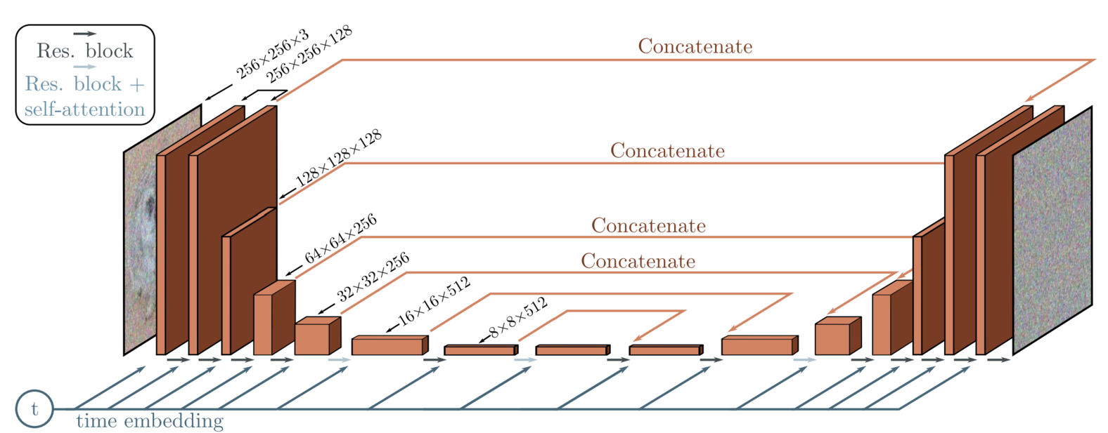
The trained neural network backbone is a UNet, as we want the input and output images to be the same size. The UNet’s goal is to predict the noise applied to the image ( x_t ). As shown in Figure 2, it consists of downsampling layers leading to a hidden layer, followed by upsampling layers, with skip connections linking corresponding layers. The UNet can receive additional information in the form of embeddings. We can provide a time embedding that indicates the expected noise level, as later time steps correspond to more noise. Additionally, we can provide a context embedding to control the generated image, such as text or depth image.

Figure 2: UNet architecture as introduced for DDPM. Image from Singh et al., 2023._

Latent Diffusion Model

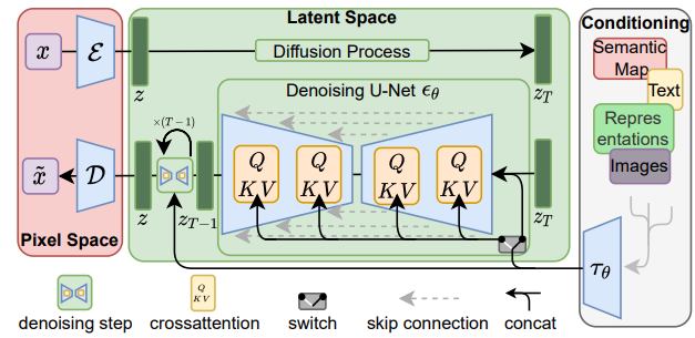
Rombach et al., 2022 introduced Latent Diffusion Model (LDM) to reduce computational demands by moving the diffusion process from the pixel space to a latent space using an autoencoder. It starts with an encoder that learns to compress the image into a latent space, then applies the diffusion and denoising processes, and finally a decoder reconstructs the image back to pixel space as shown in Figure 3. The objective is given by Equation 2.

$ L_{LDM} = E_{\varepsilon(x),\epsilon\sim N(0,1),t} [ || \epsilon - \epsilon_{\theta}(z_{t},t) ||^{2}_{2} ] $

This popular approach, introduced in Rombach et al., 2022, got the name Stable Diffusion and achieved great performance for multiple tasks.

Figure 3: Latent Diffusion Model architecture from Rombach et al., 2022._

Conditioning Mechanism

As mentioned, the UNet can receive context embeddings to control the generated image. In text-to-image tasks, it utilizes text representation using CLIP’s encoder. In this case, the learning objective is shown in Equation 3.

$ L_{LDM} = E_{\varepsilon(x), y, \epsilon\sim N(0,1),t} [ || \epsilon - \epsilon_{\theta}(z_{t},t,\tau_{\theta}(y)) ||^{2}_{2} ] $

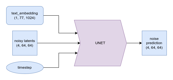
As shown in Figure 4, the UNet’s inputs are the noisy latents, timestep, and the desired condition. In text-to-image models, the condition is a text embedding created from the user’s prompt, which is fed through a text encoder to become a numerical representation.

For tasks other than text-to-image, such as inpainting, we can keep the image unchanged except for a specific region indicated by an input mask. This mechanism is very important for the editing part. We can see how the attention mechanism, together with the diffusion model, allows us to add more conditioning, not just text embedding but also masks.

Figure 4: Conditioning mechanism: shows how the UNet can use the text embedding, Image from Hugging Face Course.

In summary, a classic text-to-image model consists of four important building blocks that assist in the sampling process. First, the user provides a prompt, which is transformed into a text embedding using a tokenizer and text encoder. Second, random noise is generated as the starting latent. Third, we iterate through a number of inference steps; at each step, we predict the noise using the trained UNet, which takes the latent, time step, and text embedding as inputs. This predicted noise helps compute the previous noisy sample and can be manipulated for additional guidance. Finally, the loop repeats until we obtain the final latent, which is then decoded into an image using a VAE decoder, transforming the compressed representation into an image.

DDIM Inversion

Since the sampling process removes noise gradually, it might take several hundred steps to generate a new image. Song et al., 2022 proposed Denoising Diffusion Implicit Models (DDIM), which can skip steps during generation and thereby speed up the denoising process. Unlike DDPM, which relies on Markov Chain behavior, DDIM removes this behavior. As a deterministic sampler, DDIM ensures that the output from the same noise input will always be the same image. This led to the task of inversion: given an image and a trained denoiser, determining the initial noise that can be denoised into that specific image. DDIM Inversion is important in the task of image editing and is used in our experiment during the inference step.

References

• Dhariwal, P., & Nichol, A. (2021). Diffusion models beat GANs on image synthesis. Advances in Neural Information Processing Systems. URL or DOI.
• Ho, J., Jain, A., & Abbeel, P. (2020). Denoising Diffusion Probabilistic Models. Advances in Neural Information Processing Systems. URL or DOI.
• Sohl-Dickstein, J., Weiss, E., Maheswaranathan, N., & Ganguli, S. (2015). Deep Unsupervised Learning using Nonequilibrium Thermodynamics. International Conference on Machine Learning. URL or DOI.
• Rombach, R., Blattmann, A., Lorenz, D., Esser, P., & Ommer, B. (2022). High-Resolution Image Synthesis with Latent Diffusion Models. Computer Vision – ECCV 2022. URL or DOI.
• Singh, A., & Anand, D. (2023). Understanding UNet: A Detailed Study on Image Segmentation Architecture. Journal of Visual Communication. URL or DOI.
• Song, J., Meng, C., & Ermon, S. (2022). Denoising Diffusion Implicit Models. International Conference on Learning Representations. URL or DOI.
• Hugging Face Course. (2023). Diffusion Models: Theory and Practice. Hugging Face, Inc.. URL or DOI.