Diffusion Models Extensions
Published:
Diffusion Models Extensions
It is good to think about what kind of problem we want to solve. If it involves image-to-image (img2img) tasks, we can take inspiration from super-resolution, colorization, and inpainting, as well as pixel-level image understanding tasks. Then, we should consider task-specific architecture customizations, changes to hyperparameters, or modifications to the loss function. Over the spatial composition of the image; precisely expressing complex layouts, poses, shapes, and forms can be difficult via text prompts alone.
Here I will explore several popular Diffusion Model (DM) Extensions:
- ControlNet
- Blended Latent Diffusion
- Palette
- SpaText
- DiffEdit
- Prompt-to-Prompt
- Fine-Tuning/Optimization Methods
1. ControlNet
Paper: Adding Conditional Control to Text-to-Image Diffusion Models
ArXiv Link: https://arxiv.org/abs/2302.05543
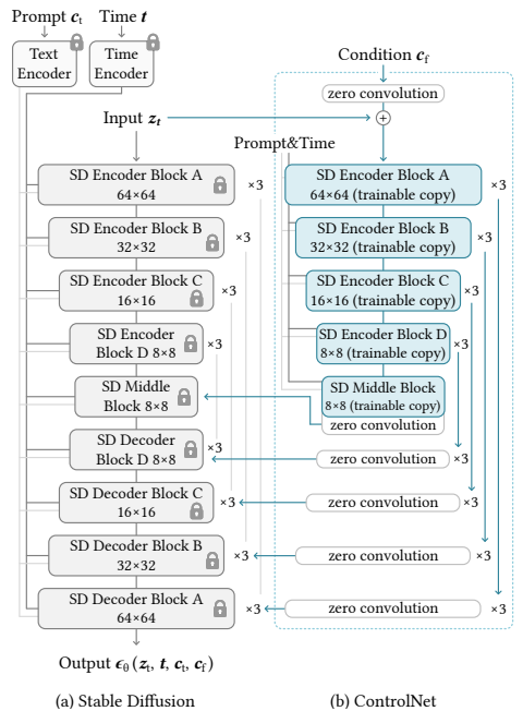
controlnet want to provide the spatial composition to txt to image diffusion models.
so they use the model trained on bilion of images, locked it, and added trainable copy.
the pre trained locked model and the trainable copy are connected via zaro convulotion.
zero convulotion layed are initialized to zero and grow during the training, ensures that the initial outputs are identical to those of the pre-trained model.
only the incremental changes (residuals) are learned. this prevent hanmful noise to affect the finetuning.
fintuning large model is not an easy task and the second part of this blog post will explore these methods.
the locked copy is efficient cuz then we dont need to save a space for the original gradients.
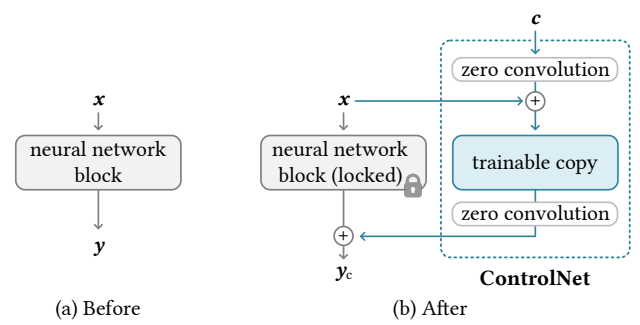
Suppose F(·; Θ) is such a trained neural block, with parameters Θ, that transforms an input feature map x, into another feature map y as y = F(x; Θ).
we lock the parameters Θ of the original block and create a trainable copy with parameters Θc.
The trainable copy takes an external conditioning vector c as input.
The trainable copy is connected to the locked model with zero convolution layers, denoted Z.
is a 1 × 1 convolution layer with both weight and bias initialized to zeros, while it might sound like it will stay zero forever they explain why it is not here.
they use two instances of zero convolutions with parameters Θz1 and Θz2.
The complete ControlNet then computes yc = F(x; Θ) + Z(F(x + Z(c; Θz1); Θc); Θz2),
where yc is the output of the ControlNet block.
2. Blended Latent Diffusion
Paper: Not yet specified
ArXiv Link: Not available
Blended latent Diffusion want to solve the problem where the user give the image, a text and a mask of the desired edited region.
formally, Given an image 𝑥, a guiding text prompt 𝑑 and a binary mask 𝑚 that marks the region of interest in the image, our goal is to produce a modified image 𝑥ˆ, s.t. the content 𝑥ˆ ⊙ 𝑚 is consistent with the text description 𝑑, while the complementary area remains close to the source image, i.e., 𝑥 ⊙ (1−𝑚) ≈ 𝑥ˆ ⊙ (1−𝑚), where ⊙ is element-wise multiplication. Furthermore, the transition between the two areas of 𝑥ˆ should ideally appear seamless.
denote foreground (fg) the modified part, background (bg) the remaining part.
We downsample the input mask 𝑚 to these spatial dimensions to obtain the latent space binary mask 𝑚 latent.
input image 𝑥 is encoded into the latent space.
we noise the initial latent 𝑧init to the desired noise level (in a single step) and manipulate the denoising diffusion process in the following way:
at each step, we first perform a latent denoising step, conditioned directly on the guiding text prompt 𝑑, to obtain a less noisy foreground latent denoted as 𝑧fg, while also noising the original latent 𝑧init to the current noise level to obtain a noisy background latent 𝑧bg.
The two latents are then blended using the resized mask, i.e.
𝑧fg ⊙ 𝑚latent + 𝑧bg ⊙ (1 − 𝑚latent),
to yield the latent for the next latent diffusion step.
at each denoising step the entire latent is modified, but the subsequent blending enforces the parts outside 𝑚latent to remain the same.

background preservation
How to keep the unchanged areas good?
1) Naïve stitching: Stitch the original image and the edited result 𝑥ˆ at the pixel level, using the input mask 𝑚. The unmasked areas were not generated by the decoder, so it does not blend seamlessly with the surrounding background.
2) Poisson image blending: Perform seamless cloning between the edited region and the original image. This often results in a noticeable color shift of the edited area. For Poisson image blending [Pérez et al. 2003], we used the OpenCV [Bradski and Kaehler 2000] implementation.
3) Latent optimization: Given the input image 𝑥, the mask 𝑚, and the edited image 𝑥ˆ, along with its corresponding latent vector 𝑧0, one could use latent optimization to search for a better vector 𝑧∗, s.t. the masked area will be similar to the edited image 𝑥ˆ and the unmasked area will be similar to the input image 𝑥. However, it cannot capture the high-frequency details, so maybe the expressivity of the decoder 𝐷(𝑧) is limited.
4) Fine-tuning decoder’s weights 𝜃 per image: Fine-tune the decoder’s weights 𝜃 on a per-image basis and use these weights to infer the result 𝑥∗ = 𝐷𝜃∗ (𝑧0).
This method yields the best result: the foreground region follows 𝑥ˆ, while the background preserves the fine details from the input image 𝑥, and the blending appears seamless.
• For latent optimization and weights optimization, we used Adam optimizer [Kingma and Ba 2014] with a learning rate of 0.0001 for 75 optimization steps per image.

3. Palette
Paper: Palette: Image-to-Image Diffusion Models
ArXiv Link: https://arxiv.org/abs/2111.05826
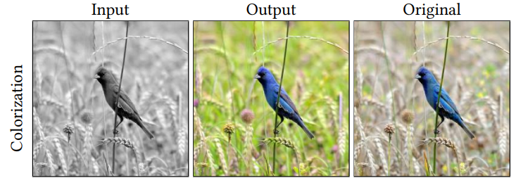
This work focuses on image-to-image tasks such as colorization, inpainting, uncropping, and more.
It is inspired by [Saharia et al. 2021]: Image Super-Resolution via Iterative Refinement.
What they did is adding in concatenation the image 𝑥 to the noisy image 𝑦𝑒.
So to my understanding, if the noise is 3 channels and the grayscale is 1 channel, the architecture is being adjusted to input of 4 channels.
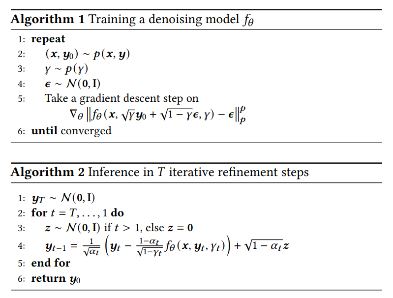
| Formally, image-to-image diffusion models are conditional diffusion models of the form 𝑝(𝒚 | 𝒙), where both 𝒙 and 𝒚 are images, e.g., for a colorization task, 𝒙 is a grayscale image and 𝒚 is a color image. |
Given a training output image 𝒚, we generate a noisy version 𝒚𝑒 and train a neural network 𝑓𝜃 to denoise 𝒚𝑒 given 𝒙 and a noise level indicator 𝛾, for which the loss is:

𝑝 is 1 or 2, depending if we want 𝐿1 or 𝐿2 norm.
- 𝐿1 yields lower diversity but reduces potential hallucination.
- 𝐿2 captures the output distribution more faithfully.
4. SpaText
Paper: SpaText: Spatio-Textual Representation for Controllable Image Generation
ArXiv Link: Not yet specified
5. DiffEdit
Paper: DiffEdit: Diffusion-Based Semantic Image Editing with Mask Guidance
ArXiv Link: DIFFEDIT
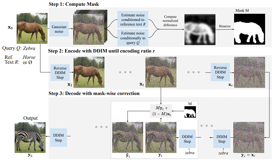
DiffEdit wants to edit an image by text only, without asking the user to provide a mask like other methods.
But since they want to preserve the background, they want to find automatically the mask of the desired edited region in the image.
So in the first step, they add 50% Gaussian noise to the image, and they denoise it with the original prompt and with the target prompt.
They take the noise estimates of these two denoising results and calculate their difference and binarize it to get a mask.
The idea is that the noise estimate of “horse” will be spatially similar to “zebra,” which will give us the animal body as the mask.
Then they use the DDIM Inversion technique to find the noise 𝑥𝑟 that will yield the original image 𝑥𝑡.
Then they take the noisy encoded image and denoise it, while injecting the mask to control the denoising,
by ˜𝑦𝑡 = 𝑀𝑦𝑡 + (1−𝑀)𝑥𝑡,
𝑥𝑡 is the inferred latent from 𝑥𝑟, 𝑀 is the mask, 𝑦𝑡 is the denoised image, so 𝑀𝑦𝑡 is the edited region, and 𝑦𝑡~ is the edited image.
6. Prompt-to-Prompt
Paper: Prompt-to-Prompt Image Editing with Cross-Attention Control
ArXiv Link: Not yet specified
Prompt-to-Prompt is an image editing framework that uses only the target text (doesn’t provide any mask). The idea is to preserve the areas where there isn’t a change between the source prompt and target prompt.
The key observation is that the connection between the text embedding and the spatial layout is in the cross-attention maps.
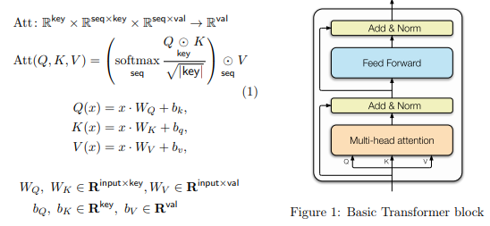
They say that in the denoising process, the text embedding is the 𝐾,𝑉 matrices, and the deep spatial features of the image are the 𝑄 matrix.
Considering that the attention is given by:
𝑀 = Softmax(Q𝐾𝑇 /√𝑑)
The cross-attention output is ϕb(𝑧𝑡) = 𝑀𝑉. We can look at 𝑀 as the similarity matrix of text and image, and 𝑉 as the values, so 𝑀𝑉 expresses the weighted average of the values.
They observed that each token in the prompt gets a corresponding cross-attention map that shows the spatial layout of that token in the image.
They observed that each token in the prompt gets a corresponding cross-attention map that shows the spatial layout of that token in the image.
So, for example, for swapping words, if we have the image and the source prompt, we can find its cross-attention maps for the words that are different in the target prompt.
Then in the denoising process, we can inject the original image cross-attention map 𝑀𝑡, overriding the 𝑀∗𝑡, to control the denoising process.


Other methods for text-conditioned image editing:
- Song et al. (2021): Proposed to condition the generation process by copy-pasting pixel values from the reference image at each denoising step.
- Nichol et al. (2021): Used a similar technique by copy-pasting pixels in the estimated final version of the image.
- Wang et al. (2022b): Used DDIM encoding of the input image and then decoded on edited sketches or semantic segmentation maps.
- The gradient of a CLIP score can also be used to match a given text query inside a mask, as in blended diffusion.
- DiffusionCLIP (Kim & Ye, 2021): Updated the weights of the diffusion model themselves via gradient descent from a CLIP loss with a target text.
Fine-Tuning and Optimization Methods
Why is fine-tuning an interesting problem for large generative models?
The direct fine-tuning or continued training of a large pre-trained model with limited data may cause overfitting and catastrophic forgetting. Researchers have shown that such forgetting can be alleviated by restricting the number or rank of trainable parameters.
Designing deeper or more customized neural architectures might be necessary for handling in-the-wild conditioning images with complex shapes and diverse high-level semantics.
One way to fine-tune a neural network is to directly continue training it with the additional training data. But this approach can lead to:
- Overfitting
- Mode collapse
- Catastrophic forgetting
Extensive research has focused on developing fine-tuning strategies that avoid such issues, including:
- HyperNetwork
- Adapter
- Additive Learning
- Low-Rank Adaptation (LoRA)
- Zero-Initialized Layers (used in ControlNet)
1. LoRA
Paper: Scaling Down to Scale Up: A Guide to Parameter-Efficient Fine-Tuning
ArXiv Link: Not yet specified
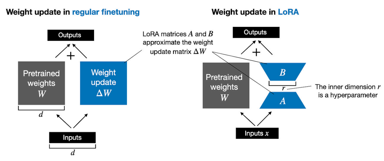
LoRA uses the idea of reparameterizing the weights of the network using a low-rank transformation. This decreases the trainable parameter count while still allowing the method to work with high-dimensional matrices, such as the pre-trained parameters of the networks.
How It Works:
Parameter update for a weight matrix in LoRA is decomposed into a product of two low-rank matrices:
𝛿𝑊 = 𝑊𝐴𝑊𝐵, 𝑊𝐴 ∈ ℝ^(𝑖𝑛×𝑟), 𝑊𝐵 ∈ ℝ^(𝑟×𝑜𝑢𝑡)
All pre-trained model parameters are kept frozen, and only 𝑊𝐴 and 𝑊𝐵 matrices are trainable. The scaling factor is constant and typically equals 1/𝑟.
After training, they can be integrated into the original 𝑊 by just adding the matrix 𝑊𝐴𝑊𝐵 to the original matrix 𝑊.
Applications:
- In Transformers, LoRA is typically used for 𝑊𝐾 and 𝑊𝑉 projection matrices in multihead attention modules.
- To achieve the best performance, it’s best to apply LoRA to all weight matrices in the model.
- In Stable Diffusion fine-tuning, LoRA can be applied to the cross-attention layers that relate the image representations with the prompts that describe them.
Additional References to Add Later
- Catastrophic Forgetting: Towards Data Science
- Cascaded Diffusion Models for High Fidelity Image Generation (Ho et al., 2021): Introduces cascaded diffusion, which comprises a pipeline of multiple diffusion models that generate images of increasing resolution for high-fidelity image synthesis.
- Classifier-Free Diffusion Guidance (Ho et al., 2021): Shows that you don’t need a classifier for guiding a diffusion model by jointly training a conditional and an unconditional diffusion model with a single neural network.
- Hierarchical Text-Conditional Image Generation with CLIP Latents (DALL-E 2) (Ramesh et al., 2022): Uses a prior to turn a text caption into a CLIP image embedding, after which a diffusion model decodes it into an image.
Techniques for Injecting Conditions into Diffusion Models
Incorporating conditions into diffusion models is crucial for guiding the generative process. This document organizes popular methods into two main categories: Layer Fusion and Attention Injection. Each approach includes explanations, advantages, and applications.
1. Layer Fusion
1.1. Element-Wise Operations
a. Addition
- How It Works: Corresponding elements of the feature maps are summed. [ F_{\text{fused}} = F_1 + F_2 ]
- Advantages:
- Simple and computationally efficient.
- Preserves spatial alignment.
- Applications:
- Residual connections (e.g., ResNet).
- Combining features in U-Net and ControlNet architectures.
b. Multiplication
- How It Works: Element-wise product of feature maps. [ F_{\text{fused}} = F_1 \odot F_2 ]
- Advantages:
- Emphasizes regions where both feature maps have high activation.
- Useful in attention mechanisms.
- Applications:
- Feature weighting.
- Attention-based architectures.
c. Maximum/Minimum
- How It Works: Takes the maximum or minimum value element-wise. [ F_{\text{fused}}(i, j) = \max(F_1(i, j), F_2(i, j)) ]
- Advantages:
- Retains the most salient features.
- Adds robustness to noise.
- Applications:
- Strong feature selection in object detection and segmentation.
1.2. Concatenation
- How It Works: Feature maps are concatenated along the channel dimension. [ F_{\text{fused}} = \text{Concat}(F_1, F_2) ] For feature maps of size (H \times W \times C_1) and (H \times W \times C_2), the fused map is (H \times W \times (C_1 + C_2)).
- Advantages:
- Retains all information from both feature maps.
- Flexible for multi-modal inputs.
- Applications:
- Skip connections in U-Net.
- Multi-scale feature fusion in Feature Pyramid Networks (FPN).
1.3. Weighted Sum
- How It Works: Feature maps are linearly combined with weights. [ F_{\text{fused}} = \alpha F_1 + \beta F_2 ]
- Advantages:
- Provides flexibility to prioritize one feature map over the other.
- Effective for balancing multi-modal inputs.
- Applications:
- Multi-task learning.
- Attention-weighted feature fusion.
1.4. Convolution-Based Fusion
- How It Works: Feature maps are concatenated and passed through a convolutional layer to learn dynamic fusion.
- Advantages:
- Reduces dimensionality while retaining useful information.
- Learns feature interactions dynamically.
- Applications:
- U-Net++ for segmentation tasks.
- RGB and depth fusion in multi-modal architectures.
1.5. Multi-Scale Fusion
- How It Works: Combines feature maps at different resolutions.
- Advantages:
- Captures both global context and fine-grained details.
- Useful for hierarchical representation learning.
- Applications:
- Feature Pyramid Networks (FPN).
- HRNet for semantic segmentation.
1.6. Bilinear Pooling
- How It Works: Computes outer products of feature vectors across the feature maps.
- Advantages:
- Captures complex feature interactions.
- Effective for fine-grained image recognition.
- Applications:
- Multi-modal fusion tasks.
- Scene graph generation.
2. Attention Injection
2.1. Cross-Attention
- How It Works: Conditions (e.g., text embeddings) are used as keys and/or values in the attention mechanism. Queries ((Q)) come from the input. [ \text{Attention}(Q, K, V) = \text{Softmax}\left(\frac{QK^T}{\sqrt{d_k}}\right)V ]
- Advantages:
- Aligns semantic and spatial features effectively.
- Allows precise control over the generation.
- Applications:
- Stable Diffusion: Text embeddings guide generation.
- Prompt-to-Prompt: Modifies cross-attention maps for editing.
2.2. Channel Attention
- How It Works: Learns to emphasize or suppress specific channels using global pooling and weighting.
- Advantages:
- Highlights critical features while suppressing noise.
- Improves model performance for complex tasks.
- Applications:
- SENet (Squeeze-and-Excitation Networks): Re-weights channel features dynamically.
2.3. Spatial Attention
- How It Works: Computes attention weights for each spatial location in the feature map.
- Advantages:
- Focuses on relevant spatial regions.
- Enhances accuracy in segmentation tasks.
- Applications:
- Spatial attention mechanisms in transformer models.
- Image segmentation tasks like SegFormer.
2.4. Mask-Guided Attention
- How It Works: A mask is used to modulate attention scores directly, ensuring focus on specific regions. [ \alpha_{ij}’ = \alpha_{ij} \cdot \text{Mask}_{ij} ]
- Advantages:
- Restricts attention to important regions.
- Helps in image-to-image translation tasks.
- Applications:
- Masked self-attention in segmentation models.
- ControlNet for spatially-guided image generation.
2.5. Conditional Cross-Attention
- How It Works: Instead of standard self-attention, cross-attention is employed where the condition (e.g., a segmentation mask) is treated as the key and/or value.
- Advantages:
- Enables effective guidance with external conditions.
- Provides fine-grained control over the output.
- Applications:
- ControlNet: Fuses segmentation maps with image features.
- DETR (Detection Transformer): Object queries as conditions in cross-attention layers.
References to Notable Works
- ControlNet: Zhang et al. (2023) - Adding Conditional Control to Text-to-Image Diffusion Models.
Paper Link - Prompt-to-Prompt: Hertz et al. (2022) - Prompt-to-Prompt Image Editing with Cross-Attention Control.
Paper Link - U-Net: Ronneberger et al. (2015) - U-Net: Convolutional Networks for Biomedical Image Segmentation.
Paper Link - SENet: Hu et al. (2018) - Squeeze-and-Excitation Networks.
Paper Link - DETR: Carion et al. (2020) - End-to-End Object Detection with Transformers.
Paper Link
