Feature Matching: From SIFT to Transformers
Published:
Draft Mode
Feature matching: From SIFT to Transformers
Introduction
For every student taking computer vision class one of the most popular algorithms is SIFT, SIFT is Great well known algoirthm and it opens your mind regarding how can you solve problems and taking consideration as scale, rotation, brigtness into account and find creative solutions. SIFT is from 2004 and since then the urge of deep learning arrived and from 2021 the transformers that took advantages of the GPUs parallilism.
In this article we will explore some of the most populr evolutions to feature matching, starting from classic computer vision algorithms as SIFT till nowaday transformers as LoFTR. I will reference all and hopefully next post I will show you my own expiriments.
The classical computer vision having 3 steps, feature detection, feature desciptors and matching. We can divide feature matching algorithm to detection based, detection free, classical computer vision, learning based algorithm and finally using transformers. In addition we will explore the step of the matching itself.
general approach of feature matching is divided to 3 steps, feature detection, feature description and feature matching. these step have been changed over the time as we will see in this article. Image from stanford slides here
Feature Matching
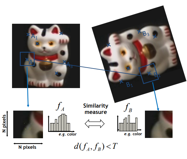
feature matching is the problem of finding correspondences between two images. for example
can you think about the challenges we are facing solving this problems? let me raise some questions, what if the rotation of the scene between the images are very strong, what is there are brightness differences, in one image the scene is brighter than the other? what if there are a lot of areas that look the same, as clear blue sky or white wall?
to solve this many of intresting algorithms trying to overcome these problems in effiencient and robust way.
the application for feature matching are a lot, everything related to 3d reconstruction, stiching images to create panorama, recognition of objects or scene and much more, i leave this to the readers to find out.
SIFT
i will do a review of sift, if you learnt it before it will be enough but if its your first time i recommand highly informative explantation such as…
the idea behind sift is as follows: we first want to detect intrest points. intrest point are mainly corners, because corners produce strong, unique gradients in multiple directions, making them distinct. the problem with corners is that if you’re zooming in, the corner may seem like a line, and we want to be robust for scale, so called scale-invariant. how can we solve it? we need to find a function where we could find the corners in the image in all kinds of scales. so we are applying Gaussian kernel on the image with kernel that is increasing, resulting in the image in different scales. then we are substracting these filtered images and the result is called DoG, difference of gaussians DoG(x,y,σ)=G(x,y,kσ)−G(x,y,σ). Gaussian blurring removes high-frequency components (e.g., fine details, noise) from an image. By subtracting one blurred image from another, the difference isolates the higher-frequency information that corresponds to edges, corners, and fine structures. DoG enhances regions with rapid intensity changes while suppressing low-frequency regions. look at the example image.

We can see in this image that at different resolutions of kernel size we see different fine details of the image:we can capture keypoints at varying scales. The DoG function enhances regions with rapid intensity changes and suppresses smooth, low-frequency areas. These changes can occur in two ways: A rapid increase in intensity (bright feature surrounded by dark areas). A rapid decrease in intensity (dark feature surrounded by bright areas).
SIFT is looking for the local maximum in DoG, because if it is a local maximum of DoG it means it is good intrest point.
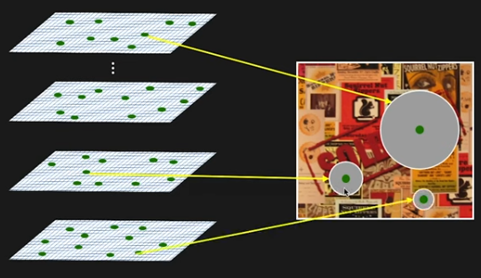
| **at the end of this detection step we will get smt like in this image, different blob size correscponds to finding the corner in different scale. We see these as blobs detection, the scale effect the size of the blob (a great video here by [First Priniciles of Computer Vision](Overview | SIFT Detector)** |
now that we have these intrest point for each of the images, remember our goal is to match features, in order to match the features we need to find a way to describe them and then do the matching. so we take the intrest point and we take a grid on it we calculate for each pixel in this grids its gradients. the gradients have oreintation and magnitude, since we want to keep the descriptor invariant to brigtness we ignore the magnitude. the orientation computed by: Theta = arctan(d I/ d y \ dI/dx) we put these orientation of the gradient on histogram, for each orientation we put the number of pixels in the area corresponding to this orientation. it is worth mentioning, that the orientation with the maximum pixels tell us the principle orientation for that blob which makes our algorithm rotation invariant cuz we edscribe the orientation compared to it. the result is descriptor which is a histogram of length 128 for each intrest point.
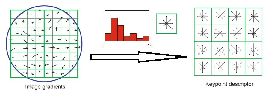
The blue is the area of the blob.So for each blob we take the first qurdrant which is 4x4 matrix and put the gradients and the number of pixel of each, and we do this for each quardarant and concatentaing these histogram to each other.
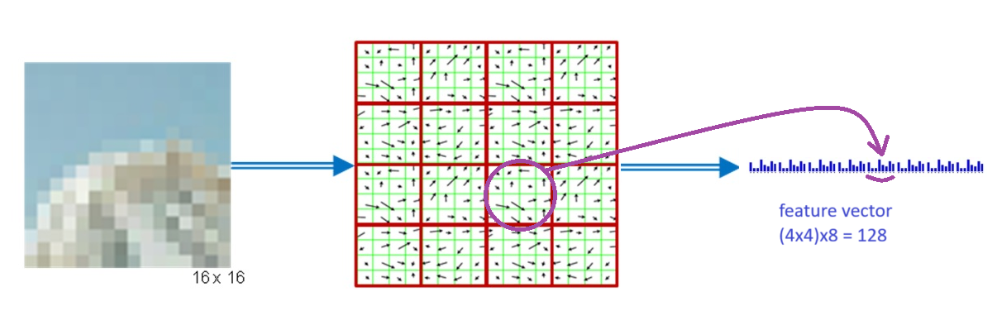
8 orientation bins from 0 to 2pi per histogram and a 4x4 histogram array. So a SIFT descriptor is a length 128 vector.Image adapted from amazing cv blog
now its time for the last step, the matching itself! remember knn, k-nearest neighbors? lets say we have a new sample of a dog information and we want to know its breed, we can look at its 3 nearest nieghbors regrading the specific known feature like its size or color, and deduce by taking the majority breed of these neightbors. we are doing the same here, we have feature descriptor in image 1 and we want to find its corrrespondence in image 2 so we are calculating the euclidean distance of each descriptor from the other descriptors in image 2, looking for the descriptor that is the much alike. remember the descriptor is a histogram so we are looking at the k closest histograms. in total we are doing #(num_of_descriptors_in_img1*num_of_descriptors_in_img2) comparisons. this kind of matcher is the brute force matcher. There is also other type of matcher which is the FLANN and mutual nearest neighbhors. a good explanation can be found in here too article . we can also apply ratio test that filter matches that there distance is above a certain threshold.
now that we reviewed SIFT, do you know any other succeeding of it? SURF introduced faster method by replacing the DoG in the feature detection phase with Hessian matrix. Later on, ORB over preform them in faster keypoint detection, compact binary feature descriptors and faster matching by using hamming distance.
but these were still using the same approach of 3 phases: Detection, Descrition and Matching.
so in 2008, SIFT Flow were introduced for dense correspondences indroducting detector-free approach.
SIFT Flow
In the classic approach but detector free: SIFT Flow: Dense Correspondence across Scenes and its Applications
From the paper: Inspired by optical flow methods, which are able to produce dense, pixel-to-pixel correspondences between two images, we propose SIFT flow, adopting the computational framework of optical flow, but by matching SIFT descriptors instead of raw pixels. In SIFT flow, a SIFT descriptor [5] is extracted at each pixel to characterize local image structures and encode contextual information. A discrete, discontinuity preserving, flow estimation algorithm is used to match the SIFT descriptors between two images. The use of SIFT features allows robust matching across different scene/object appearances and the discontinuity-preserving spatial model allows matching of
From https://people.csail.mit.edu/celiu/SIFTflow/
For every pixel in an image, we divide its neighborhood (e.g. 16×16) into a 4×4 cell array, quantize the orientation into 8 bins in each cell, and obtain a 4×4×8=128-dimensional vector as the SIFT representation for a pixel. We call this per-pixel SIFT descriptor SIFT image.
We formulate SIFT flow the same as optical flow with the exception of matching SIFT descriptors instead of RGB values.
The energy function for SIFT flow is defined as:
sift_flow_objective.png
which contains a data term, small displacement term and smoothness term (a.k.a. spatial regularization). The data term on line 1 constrains the SIFT descriptors to be matched along with the flow vector w(p). The small displacement term on line 2 constrains the flow vectors to be as small as possible when no other information is available. The smoothness term on line 3 constrains the flow vectors of adjacent pixels to be similar. In this objective function, truncated L1 norms are used in both the data term and the smoothness term to account for matching outliers and flow discontinuities, with t and d as the threshold, respectively. We use a dual-layer loopy belief propagation as the base algorithm to optimize the objective function.
One big difference between optical flow and SIFT flow is that the search window size for SIFT flow is much larger since an object can move drastically from one image to another in scene alignment. Therefore, we need to design efficient algorithm to cope with the complexity. In SIFT flow, a pixel in one image can literally match to any pixels in the other image. To address the performance drawback, we designed a coarse-to-fine SIFT flow matching scheme roughly estimate the flow at a coarse level of image grid, then gradually propagate and refine the flow from coarse to fine. A SIFT pyramid {s(k)} is established At each pyramid level
searching window After BP converges, the system propagates the optimized flow vector w(p3) to the next (finer) level to be c2 where the searching window of p2 is centered. That pyramimd take the computation from O(h^4) to O(H^2LOGH). h^2 is the number of pixels in image.
the start of deep learning area can be subjected to the success of AlexNet in 2012 for classification task, that showed the usage of large dataset and GPUs. since then deep learning methods overcome preformances in a lot of classic computer vision task and so it also been used for feature matching task. mentionable works are MatchNet DeepDesc and LIFT. here we will explore SuperPoint from 2018.
SuperPoint
SuperPoint: Self-Supervised Interest Point Detection and Description self-supervised framework for training interest point detectors and descriptors . our fully-convolutional model operates on full-sized images and jointly computes pixel-level interest point locations and associated descriptors in one forward pass. We introduce Homographic Adaptation, a multi-scale, multihomography approach for boosting interest point detection repeatability and performing cross-domain adaptation (e.g., synthetic-to-real). we create a large dataset of pseudo-ground truth interest point locations in real images, supervised by the interest point detector itself To generate the pseudo-ground truth interest points, we first train a fully-convolutional neural network on millions of examples from a synthetic dataset we created, consists of simple geometric shapes with no ambiguity in the interest point locations. MagicPoint performs surprising well on real images despite domain adaptation difficulties [7]. To bridge a gap in performance on real images, we developed a multi-scale, multi-transform technique − Homographic Adaptation We use Homographic Adaptation in conjunction with the MagicPoint detector we named the resulting detector SuperPoint.
superpoint_decoders.png
The encoder is VGG-style [27] encoder to reduce the dimensionality of the image. The encoder maps the input image I to an intermediate tensor B. The output of the encoder goes to Interest Point Decoder and Descriptor decoder. For interest point detection, each pixel of the output corresponds to a probability of “point-ness” for that pixel in the input. The Descriptor Decoder output a dense map of L2- normalized fixed length descriptors. The final loss is the sum of two intermediate losses: one for the interest point detector, Lp, and one for the descriptor, Ld. What I still don’t understand is the magic point and homographic adaptation are being trained, just so we could get labeled data and on this labeled data train the superpoint network?
How to choose intresting point? So they did a sytentic lie quds, cubes, stars etc. bilion on this examples. It worked extramly well. But in order to move to real picture they did the homographic adaptation. They take real image, they do synthetic wrap, and run the detector, they will get point set for each homography, we wrap them back using point aggregation and they we can detect point supetset.
What good is that once we know the homography we know where the points map in the other image. So it is siamese training with pairs of images. homographies are at the core of our self-supervised approach An ideal interest point operator should be covariant with respect to homographies. We sample within pre-determined ranges for translation, scale, in-plane rotation, and symmetric perspective distortion using a truncated normal distribution. These transformations are composed together with an initial root center crop. We apply the Homographic Adaptation technique at training time to improve the generalization ability of the base MagicPoint architecture on real images.
Neighbourhood Consensus Networks
we follow the common practice of using a deep convolutional neural network (CNN) as a dense feature extractor.
Superglue
We introduce a flexible context aggregation mechanism based on attention, enabling SuperGlue to reason about the underlying 3D scene and feature assignments jointly. our technique learns priors over geometric transformations and regularities of the 3D world through end-to-end training from image pairs. Instead of learning better taskagnostic local features followed by simple matching heuristics and tricks, we propose to learn the matching process from pre-existing local features Inspired by the success of the Transformer [61], it uses self- (intra-image) and cross- (inter-image) attention to leverage both spatial relationships of the keypoints and their visual appearance.
They said previous works have architectures still requires the nn search for the matching, and if not they preform dense matching so it still put some limitation.
They said also that the importance of context, cuz for difficult scenarios is it hard to make matches using only the local information we need also the global.
superglue_formulation.png
Transformers
one of the most infuluential papers latley is Attention is all you need introducing Transformers in 2017. LoFTR introduced in 2021, inspired by SuperGlue and showcasing the usage of transformers for feature matching.
a bit about transformers. the transformer architecture contatins the self-attention mechanism. the input x is being multiplied (?) with 3 trained matrices WQ, WK, WV (implemented in pytorch as nn.Linear). the output from xWQ and xWK is being multiplied in dot product manner to produce similarity matrix and this is being through softmax to produce values ranging from 0 to 1. we usually have several Q,K,V matrices that are being processed in parallel and called attention head.
important notes:
1) multiplication of tensors - if x is of shape [B, N, C], batch size, num of tockens, channels respectively, and the Wq for instance is of shape [C, dq] where C is the Input embedding dimentions and dk is the projected query dimension. so the result will be of size [B, N, dq]. Pytorch performs batch-wise matrix multiplication when multiplying a tensor with a matrix, in practice it flatten x to [BxN, C].
2) positional encoding - we want to keep track on the sequence order, whether it is the order of words in sentences or patches in image, but the network is permutation invariant because of global avg pooling. we can just embed the vector, which is called positional embedding, or we can find a function that will encode this position information, cosince and sine are good choices cuz these function can represent an infinite range of number but their result is between [-1,1]. in the implementation it is used by nn.Embedddig(seq_len, k) which is a lookup table that stores embedings of fixed dictionary. positional embedding are important cuz the give us the spatial awarness, ensure that the matching is context-aware.
3) receptive field - f the receptive field of (a) Convolutions and (b) Transformers Different network architectures have different receptive fields. Assuming shallow architectures, convolutional neural networks (CNNs) have a smaller receptive field compared to transformers as shown in Fig. 2. In CNNs, the receptive field grows incrementally one layer after another. In transformers, however, the receptive field spans all input (tokens) after a single layer. Yet, these receptive fields’ estimates are only theoretical! From https://ahmdtaha.medium.com/understanding-the-effective-receptive-field-in-deep-convolutional-neural-networks-b2642297927e
great explanation about transformers can be found here
LoFTR
LoFTR was demonstrating three concepts that showed great performence, first is the detector free architecture, second is the usage of transformers utilizing its global context, and third is a module that refine coarse matching.
lets go over the pipeline of LoFTR,
each of the images are going thouroug cnn backbone, specifically FPN, and we use multi-level features, we use feature map which is 1/8th of the size of the original image for the coarse matching and at later point we use feature map which is 1/2 of the size of the original image. ok let proceed with the feature map that is 1/8th of the size of the original image. we are flatenning it to 1D vector and adding it with the positional encoding, the positional encoddings derived from the feature map shape and it is fixed, the goal of it is to keep the information regarding the position in the feature map. the result is getting into self attention block. in this stage each image is only processed with itself. the next step is the cross attention, in this steps the information from both images is crossed and we recived F~. you can think about it like this, we had feature maps from two images and the mission to match them is hard cuz they are looking only on their local neighborhood, the attention blocks gives us larger global context that suppose to create outputs where that matching task would be easier.
in the next step we are computing a score matrix of these transformed feature representations. then we take this score matrix and use dual-softmax to get the matrix Pc which is the confidence matrix. we are only take matches that are about a certain confidence threshold and also enforce the mutual nearest neighbor criteria which means a match between point A and B is considred only if A is the nearest neighbor of B and also B is the nearest neighobor of A.
remember i told you we use the FPN to get also feature map 1/2 of the image dimention? now we will use it in order to refine our matches. we locate each match in these feature maps and process a window of size 5x5 around each match. these windows are also transfered to attention block and then are correlated to recieved a heatmap where a pixel color representing higher probability for a match. this step allows us to get subpixel accuracy.
the trained blocks here are the CNN backbone, and the two transformers blocks, the loss is the sum of the coarse-level and the fine-level loss L = Lc +Lf.
then we had efficientLoFTR.
lets see how we improved over the years, testing challenging matching scenarios.
i am using the scenarious from kaggle’s image matching challenge 2024 , the data they procided is for 3D reconstruction, but it this notebook i will use pairs of images for the feature matching task only. i will use these pairs to compare the SIFT and LoFTR approaches for feature matching. —-
Phototourism and historical preservation: different viewpoints and occlusions 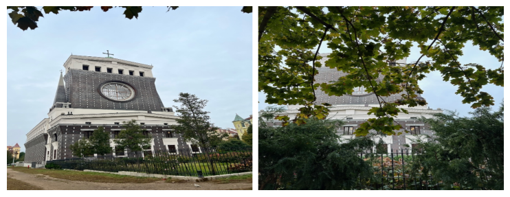
LoFTR: 
SIFT:  —-
—-
zoom 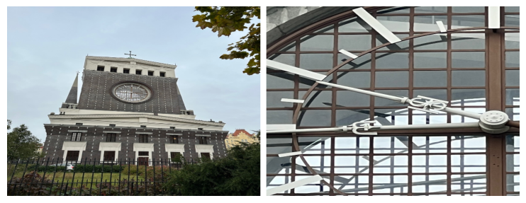
LoFTR: 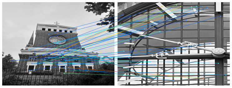
SIFT: 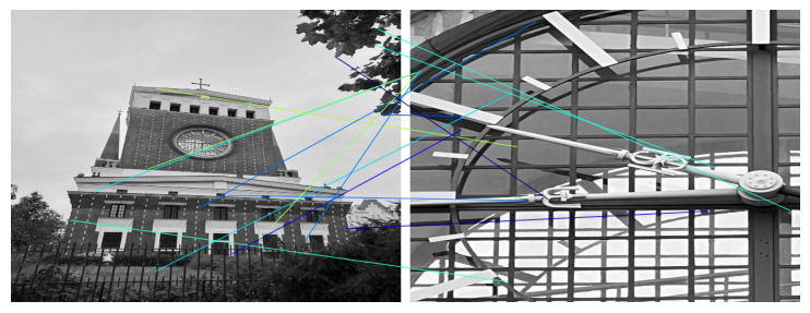
Phototourism and historical preservation sensor types, poor lighting, different time of day/year 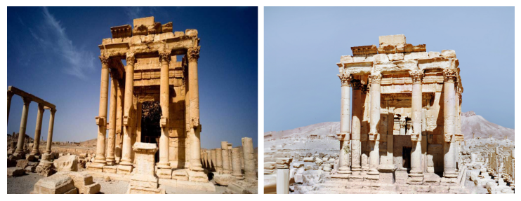
LoFTR: 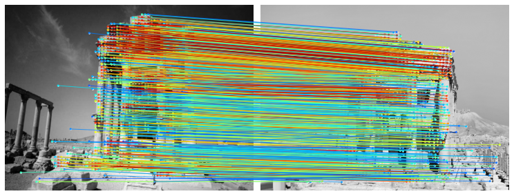
SIFT: 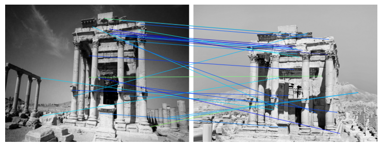 —-
—-
Aerial: images from drones, featuring arbitrary in-plane rotations, matched against similar images and also images taken from the ground 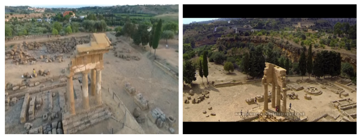
LoFTR: 
SIFT:  —-
—-
mixed aerial-ground 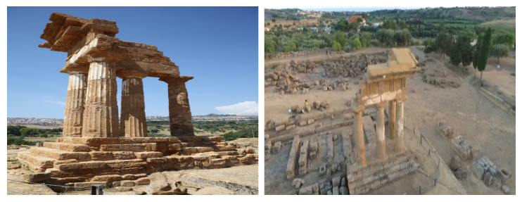
LoFTR: 
SIFT: 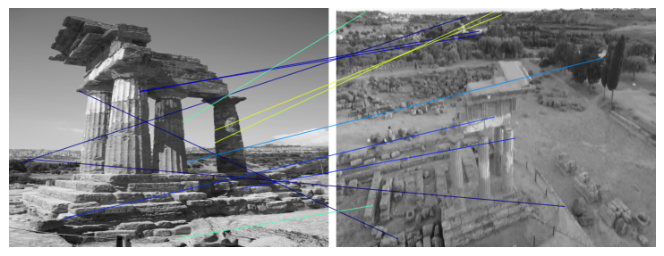 —-
—-
temporal changes photographs taken months or years apart, in different weather such in lizard: 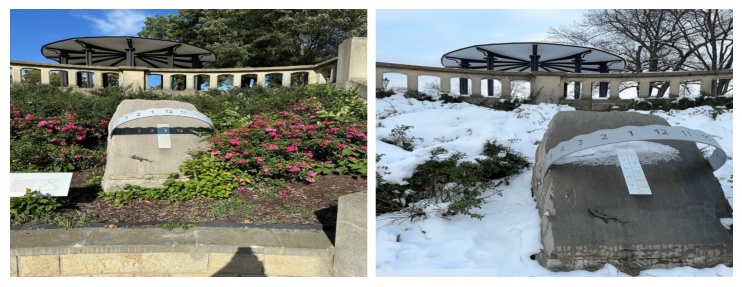
LoFTR: 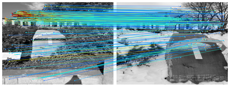
SIFT: 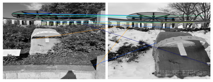
Natural environments: highly non-regular structures such as trees and foliage the pond 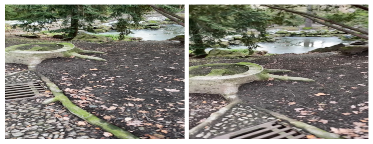
LoFTR: 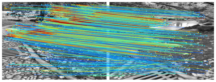
SIFT: 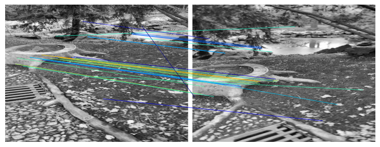
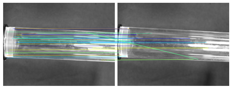
Transparencies and reflections: objects like glassware are lacking in texture and create reflections and specularities which pose a different set of problems, we can see transparent glass 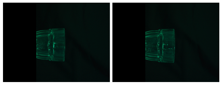
LoFTR: 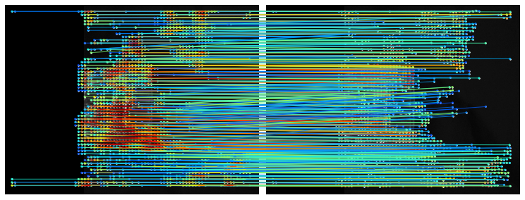
SIFT: 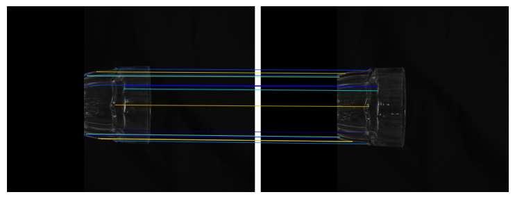
transparent 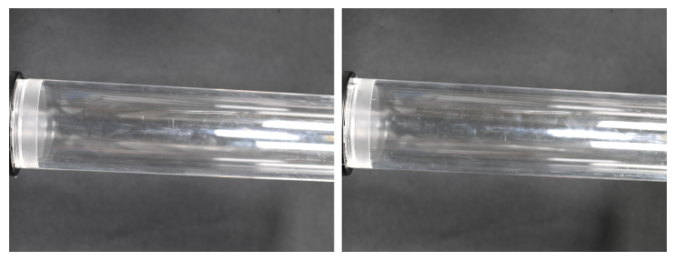
LoFTR: 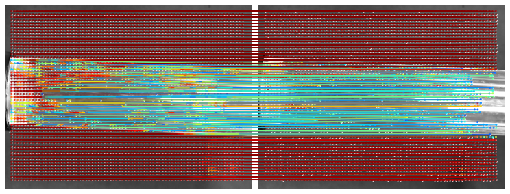
SIFT: